4 S3 Tables, Iceberg and S3 Vectors

Iceberg tables in S3 Tables, and vector search in S3 Vectors.

4.1 Before you start

Start the Iceberg catalog and the two engines, and select the oblako profile:

oblako up iceberg
oblako up s3tables
oblako up s3vectors
export AWS_PROFILE=oblako

The table listings use PyIceberg, the Python library for Iceberg:

uv add boto3 "pyiceberg[pyarrow,pandas]"

The examples keep daily page-view counts for a website, and a few pages of its documentation as vectors.

4.2 Table formats

The partitioned Parquet dataset at the end of Chapter 3 is a set of files, which works while one program writes it and others only read. It leaves three gaps: if two jobs write at once, a reader can see half of one job’s files; if you add a column, nothing records which files have it; and once a file is overwritten, the old version is gone.

Apache Iceberg is an open table format that closes these gaps with metadata. An Iceberg table is still Parquet files in object storage, plus a tree of small files that says which data files make up the table at each moment (Figure 4.1):

a catalog entry points at the table’s current metadata file;
the metadata file holds the schema, the partitioning and a list of snapshots, one per change;
each snapshot points at manifests, which list data files with statistics such as each column’s minimum and maximum.

A write adds data files, then new manifests and a new metadata file. Finally it swaps the catalog’s pointer to that metadata file in one atomic step, so a reader sees the table either as it was before the swap or as it is after it. When two writers commit at the same time, the catalog accepts only a swap made from the current metadata file; the other writer finds the table has moved on and retries its commit on the new state. An append commits on retry unless the retries run out under heavy contention; a change that conflicts with the one just committed, such as a delete of files the other writer rewrote, fails instead of overwriting it. Old snapshots remain until they are expired, so earlier versions of the table stay readable.

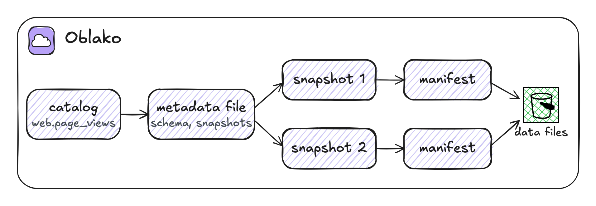
Figure 4.1: An Iceberg table. The catalog points at the current metadata file; each snapshot lists the data files it contains through manifests.

Because every engine reads the same metadata, an Iceberg table written from Python can be queried by Athena, Spark or Trino without copying it.

4.3 S3 Tables

S3 Tables is S3’s managed Iceberg service. You create a table bucket, a bucket that holds only Iceberg tables, and inside it namespaces, which group tables the way a database groups schemas. S3 Tables runs the Iceberg catalog for those tables and maintains them in the background: it compacts small files and expires old snapshots.

You work with S3 Tables through two interfaces: the s3tables API manages buckets, namespaces and tables, and the data goes through the Iceberg REST endpoint, which speaks the standard Iceberg catalog protocol that any Iceberg client supports.

What oblako runs

oblako runs one Iceberg REST catalog, tabulario/iceberg-rest, which keeps its files in oblako’s S3. In front of it, the S3 Tables engine on port 8013 serves the s3tables API and, under /iceberg, the same Iceberg endpoint AWS serves, addressed as on AWS by the table bucket’s ARN. Each table bucket becomes the first level of a namespace in the shared catalog, so the tables created here are also visible to Trino, and through Trino to Athena in the next chapter.

4.4 Creating a table bucket

The s3tables API creates the bucket and a namespace in it:

import boto3

s3tables = boto3.client("s3tables")
bucket_arn = s3tables.create_table_bucket(name="analytics")["arn"]
s3tables.create_namespace(
    tableBucketARN=bucket_arn, namespace=["web"]
)

print(bucket_arn)
namespaces = s3tables.list_namespaces(tableBucketARN=bucket_arn)
print(namespaces["namespaces"][0]["namespace"])

arn:aws:s3tables:us-east-1:123456789012:bucket/analytics
['web']

The rest of the chapter identifies the bucket by this ARN, whose account number is the simulated account from Chapter 2.

4.5 Connecting PyIceberg

PyIceberg connects to S3 Tables as a REST catalog, with the table bucket’s ARN as the warehouse and requests signed with your AWS credentials. The connection lives in a small module, catalog.py, which the later listings share:

import boto3
from pyiceberg.catalog import load_catalog


def open_catalog():
    s3tables = boto3.client("s3tables")
    buckets = s3tables.list_table_buckets(prefix="analytics")
    return load_catalog(
        "s3tables",
        **{
            "type": "rest",
            # the profile's S3 Tables endpoint, oblako or AWS
            "uri": s3tables.meta.endpoint_url + "/iceberg",
            "warehouse": buckets["tableBuckets"][0]["arn"],
            "rest.sigv4-enabled": "true",
            "rest.signing-name": "s3tables",
            "rest.signing-region": s3tables.meta.region_name,
        },
    )

PyIceberg does not read the endpoints in an AWS profile, so catalog.py takes the catalog’s URI from the boto3 client: the S3 Tables endpoint the selected profile gives, followed by /iceberg. Under the oblako profile that is oblako’s catalog, http://localhost:8013/iceberg; under an AWS profile it is the S3 Tables endpoint for your region, and catalog.py does not change.

4.6 Creating and appending to a table

PyIceberg creates a table from an Arrow schema and appends Arrow data to it:

import pyarrow as pa
from catalog import open_catalog

catalog = open_catalog()
views = pa.table(
    {
        "day": ["2026-09-01", "2026-09-01", "2026-09-02"],
        "page": ["/", "/pricing", "/docs"],
        "views": [120, 31, 45],
    }
)
schema = views.schema
table = catalog.create_table("web.page_views", schema=schema)
table.append(views)

print(catalog.list_tables("web"))
print(table.scan(row_filter="views > 40").to_pandas())

[('web', 'page_views')]
          day   page  views
0  2026-09-01      /    120
1  2026-09-02  /docs     45

append wrote a Parquet file, a manifest, a snapshot and a new metadata file, then committed them in one step. scan with a row_filter uses the column statistics in the manifests to skip files that cannot match before it reads any data.

4.7 Snapshots and time travel

Every commit creates a snapshot, and earlier snapshots remain readable:

import pyarrow as pa
from catalog import open_catalog

table = open_catalog().load_table("web.page_views")
first = table.current_snapshot().snapshot_id

more = pa.table(
    {"day": ["2026-09-03"], "page": ["/"], "views": [98]}
)
table.append(more)

for entry in table.history():
    print(entry.snapshot_id, entry.timestamp_ms)

print("now:", table.scan().to_arrow().num_rows, "rows")
then = table.scan(snapshot_id=first).to_arrow()
print("then:", then.num_rows, "rows")

7052313727309517191 1790942355646
953361004551372475 1790942356454
now: 4 rows
then: 3 rows

The table has two snapshots, and a scan pinned to the first one returns the table as it was before the second append. You can use this to reproduce an earlier report or to check what a bad write changed, without keeping copies.

4.8 Changing the schema

Iceberg tracks each column by an ID that is independent of its name and position, so adding, renaming or dropping a column changes only the metadata and leaves the data files as they are:

import pyarrow as pa
from catalog import open_catalog
from pyiceberg.types import StringType

table = open_catalog().load_table("web.page_views")
with table.update_schema() as update:
    update.add_column("country", StringType())

new = pa.table(
    {
        "day": ["2026-09-04"],
        "page": ["/docs"],
        "views": [52],
        "country": ["NL"],
    }
)
table.append(new)
rows = table.scan().to_pandas().sort_values("day")
print(rows.tail(3))

          day   page  views country
4  2026-09-02  /docs     45    None
1  2026-09-03      /     98    None
0  2026-09-04  /docs     52      NL

Rows written before the change read the new column as empty; rows written after carry it.

4.9 S3 Vectors

A vector here is a list of numbers that stands for a piece of content, such as a page of text, so that similar content has nearby vectors. An embedding model produces it, such as one of those Bedrock offers. A search by meaning finds the vectors nearest to the vector of a question.

S3 Vectors stores vectors in S3 and searches them. A vector bucket holds indexes. Each index fixes the number of dimensions and the distance measure, and holds vectors that each carry a key and optional metadata you can filter on.

The listing uses three-dimensional vectors written by hand, which stand in for the embeddings of three documentation pages:

import boto3

s3vectors = boto3.client("s3vectors")
s3vectors.create_vector_bucket(vectorBucketName="docs-vectors")
s3vectors.create_index(
    vectorBucketName="docs-vectors",
    indexName="pages",
    dataType="float32",
    dimension=3,
    distanceMetric="cosine",
)


def page(key, vector, section):
    return {
        "key": key,
        "data": {"float32": vector},
        "metadata": {"section": section},
    }


s3vectors.put_vectors(
    vectorBucketName="docs-vectors",
    indexName="pages",
    vectors=[
        page("pricing", [0.9, 0.1, 0.0], "sales"),
        page("quickstart", [0.1, 0.9, 0.2], "docs"),
        page("api", [0.0, 0.8, 0.6], "docs"),
    ],
)

resp = s3vectors.query_vectors(
    vectorBucketName="docs-vectors",
    indexName="pages",
    queryVector={"float32": [0.1, 1.0, 0.3]},
    topK=2,
    filter={"section": "docs"},
    returnDistance=True,
    returnMetadata=True,
)
for hit in resp["vectors"]:
    print(hit["key"], round(hit["distance"], 4), hit["metadata"])

quickstart 0.0027 {'section': 'docs'}
api 0.0656 {'section': 'docs'}

The query asks for the two nearest vectors in the docs section. Cosine distance is one minus the cosine of the angle between two vectors, so 0 means the two vectors point the same way, and quickstart, at 0.0027, is almost parallel to the query. pricing is further away, and the metadata filter excludes it as well.

4.10 Where oblako differs from AWS

One catalog. oblako keeps every table bucket in one Iceberg catalog, as the first level of a namespace, where AWS makes each table bucket its own catalog. Your code behaves the same, and Trino and Glue see oblako’s table buckets as namespaces.
No maintenance. S3 Tables compacts files and expires snapshots on its own, and oblako does neither, so snapshots and small files accumulate for as long as the table exists.
S3 Vectors searches by brute force and keeps vectors in memory, so its results are exact (AWS does not promise exact results on large indexes) and the vectors are lost when the engine stops.
Permissions are not enforced, for tables or vectors.

4.11 Running it on AWS

The listings run on AWS without code changes once you select an AWS profile; catalog.py then connects PyIceberg to the S3 Tables endpoint for your region. Your role needs the s3tables permissions for the bucket, namespace and table operations, which PyIceberg calls through the endpoint. Check that S3 Tables and S3 Vectors are available in your region. When you finish, delete the table, the namespace and the table bucket, and the vector index and vector bucket.

4.12 Summary

Iceberg adds atomic commits, snapshots and schema changes to files in object storage, through metadata that lists which files make up each version of a table. S3 Tables is a managed Iceberg service in which the s3tables API manages buckets and namespaces and any Iceberg client reads and writes through the REST endpoint, addressed by the table bucket’s ARN. S3 Vectors stores vectors with metadata and finds the ones nearest to a query. On oblako, the same code runs against one shared Iceberg catalog and a brute-force vector engine.