13 A multi-node Redshift
Distribution styles, skew and co-located joins on a Redshift cluster with several compute nodes.
13.1 Before you start
oblako up redshift
oblako up redshift-data
export AWS_PROFILE=oblako
uv add boto3 redshift-connector pyarrowoblako trust from Chapter 2 must have run in this environment, because the listings connect with certificate verification. The first cluster you create pulls oblako’s cluster image, or builds it from oblako’s sources when it cannot be pulled, which takes a few minutes; later clusters start in seconds.
13.2 Nodes, slices and distribution
A multi-node Redshift cluster has one leader node and several compute nodes. Clients connect to the leader, which plans each query, sends the work to the compute nodes and combines their results. The compute nodes store the tables, and each is divided into slices, each with its own share of the node’s memory and disk. A query runs on all slices at once, so it is as fast as the slice with the most work.
Where each row lives is decided by the table’s distribution style. KEY distribution hashes a chosen column, the distribution key, so rows with the same key value land on the same slice. ALL keeps a full copy of the table on every node, which suits small tables that many queries join to. EVEN spreads rows round-robin, and AUTO, the default, lets Redshift choose and change the style as the table grows. A sort key orders the rows within each slice, so that range filters on it can skip blocks.
Two things follow from this. A table distributed on a column with few values, or with a few very common values, puts more rows on some slices than others, and that skew makes every query on the table wait for its busiest slice. And when two tables are distributed on the column they are joined on, matching rows are already on the same slice, so the join runs without moving rows between nodes; such a join is co-located.
What oblako runs
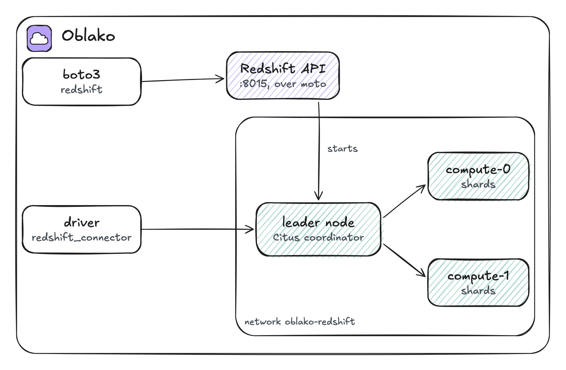
Chapter 7 ran one Redshift engine on port 5439. A cluster created through the Redshift API with ClusterType=’multi-node’ runs as several containers instead: oblako’s Redshift engine with Citus, an open-source PostgreSQL extension that shards tables across servers. The leader is the Citus coordinator and holds no table data, and each compute node is a Citus worker (Figure 13.1). The Redshift API on port 8015 is a proxy in front of moto that starts, reports and removes these containers; the cluster’s endpoint is its own name and port. Citus is licensed under the AGPL-3.0, which matters if you distribute or host a service built on the cluster image.
13.3 Creating a cluster
import boto3

redshift = boto3.client("redshift")
redshift.create_cluster(
    ClusterIdentifier="analytics",
    ClusterType="multi-node",
    NodeType="ra3.large",
    NumberOfNodes=2,
    MasterUsername="admin",
    MasterUserPassword="Analytics-local-1",
    DBName="dev",
)
waiter = redshift.get_waiter("cluster_available")
waiter.wait(ClusterIdentifier="analytics")

found = redshift.describe_clusters(ClusterIdentifier="analytics")
cluster = found["Clusters"][0]
print(cluster["ClusterStatus"], cluster["NumberOfNodes"], "nodes")
print(cluster["Endpoint"]["Address"])
for node in cluster["ClusterNodes"]:
    print(node["NodeRole"], node["PrivateIPAddress"])
available 2 nodes
analytics.us-east-1.redshift.localhost
LEADER 172.28.0.4
COMPUTE-0 172.28.0.2
COMPUTE-1 172.28.0.3NumberOfNodes counts compute nodes; the leader is extra. ClusterNodes lists every node with its role, and the endpoint is the leader’s. On AWS the cluster takes several minutes to become available, and the waiter covers both cases.
The listings connect through one helper, which looks the endpoint up by cluster identifier:
import boto3
import redshift_connector

redshift = boto3.client("redshift")


def connect(cluster_id="analytics"):
    found = redshift.describe_clusters(
        ClusterIdentifier=cluster_id
    )
    endpoint = found["Clusters"][0]["Endpoint"]
    conn = redshift_connector.connect(
        host=endpoint["Address"],
        port=endpoint["Port"],
        database="dev",
        user="admin",
        password="Analytics-local-1",
        ssl=True,
        sslmode="verify-ca",
    )
    conn.autocommit = True
    return conn


def query(sql):
    with connect().cursor() as cur:
        cur.execute(sql)
        return cur.fetchall() if cur.description else []
13.4 Loading the tables
The data is a shop’s orders, its customers and the regions they belong to, written as Parquet to S3 for COPY:
import datetime
import io
import random

import boto3
import pyarrow as pa
import pyarrow.parquet as pq

s3 = boto3.client("s3")
s3.create_bucket(Bucket="warehouse-staging")
rng = random.Random(7)
N = 20000  # orders
day0 = datetime.date(2026, 9, 1)
days = [day0 + datetime.timedelta(d) for d in range(30)]
names = "North South East West Coast Hills Lakes Plains".split()


def amount():
    return round(rng.uniform(5, 250), 2)


tables = {
    "customers": {
        "customer_id": list(range(1, 2001)),
        "region": [f"r{i % 8}" for i in range(1, 2001)],
    },
    "orders": {
        "order_id": list(range(1, N + 1)),
        "customer_id": [rng.randint(1, 2000) for _ in range(N)],
        "order_date": [days[i % 30] for i in range(N)],
        "total": [amount() for _ in range(N)],
    },
    "regions": {
        "region": [f"r{i}" for i in range(8)],
        "name": names,
    },
}
for name, columns in tables.items():
    table = pa.table(columns)
    buffer = io.BytesIO()
    pq.write_table(table, buffer)
    key = f"{name}/part-0.parquet"
    body = buffer.getvalue()
    s3.put_object(Bucket="warehouse-staging", Key=key, Body=body)
    print(name, table.num_rows, "rows")
customers 2000 rows
orders 20000 rows
regions 8 rowsThe orders and customers are distributed on customer_id, the column they are joined on, and the eight regions are copied to every node. Each table is then loaded with COPY, which reads the Parquet files on the compute nodes’ behalf:
from cluster import query

ROLE = "arn:aws:iam::123456789012:role/redshift-copy"
query("""
    CREATE TABLE customers (
        customer_id integer,
        region      varchar(4))
    DISTKEY(customer_id) SORTKEY(customer_id)""")
query("""
    CREATE TABLE orders (
        order_id    integer,
        customer_id integer,
        order_date  date,
        total       decimal(10, 2))
    DISTKEY(customer_id) SORTKEY(order_date)""")
query("""
    CREATE TABLE regions (
        region varchar(4),
        name   varchar(16))
    DISTSTYLE ALL""")
for table in ("customers", "orders", "regions"):
    query(f"""
        COPY {table} FROM 's3://warehouse-staging/{table}/'
        IAM_ROLE '{ROLE}' FORMAT AS PARQUET""")
print(query("SELECT count(*) FROM orders"))([20000],)13.5 Checking the distribution
SVV_TABLE_INFO reports each table’s distribution style, its first sort key column, its row count and its skew:
from cluster import query

rows = query("""
    SELECT "table", diststyle, sortkey1, tbl_rows, skew_rows
    FROM svv_table_info
    WHERE "table" IN ('customers', 'orders', 'regions')
    ORDER BY "table" """)
for row in rows:
    print(*row)
customers KEY(customer_id) customer_id 2000 1.03
orders KEY(customer_id) order_date 20000 1.04
regions ALL None 8 Noneskew_rows is the number of rows on the fullest slice divided by the number on the emptiest, so 1.00 is a perfectly even spread. With 2,000 distinct customer IDs hashed over the nodes, the orders are within 4% of even. The regions table has no skew value because every node holds all of it.
13.6 Choosing the distribution key
A distribution key with few distinct values spreads rows less evenly. This listing copies the orders into a table distributed on the order date, which has 30 values:
from cluster import query

query("""
    CREATE TABLE orders_by_day DISTKEY(order_date) AS
    SELECT * FROM orders""")
rows = query("""
    SELECT "table", diststyle, skew_rows
    FROM svv_table_info
    WHERE "table" IN ('orders', 'orders_by_day')
    ORDER BY "table" """)
for row in rows:
    print(*row)
orders KEY(customer_id) 1.04
orders_by_day KEY(order_date) 1.31The fullest node now holds 1.31 times the rows of the emptiest, against 1.04 for the customer key. With a key such as a country or a status code, a few values can hold most of the rows, and the skew is far larger. A good distribution key has many distinct values, spreads rows evenly, and is the column the largest tables are joined on. CREATE TABLE ... AS SELECT with a new key, as here, is also how you change the distribution of a table that already holds data.
13.7 Co-located joins
The revenue by region joins all three tables:
from cluster import query

rows = query("""
    SELECT r.name, count(*) AS orders, sum(o.total) AS revenue
    FROM orders o
    JOIN customers c ON c.customer_id = o.customer_id
    JOIN regions r ON r.region = c.region
    GROUP BY r.name
    ORDER BY revenue DESC
    LIMIT 3""")
for row in rows:
    print(*row)
East 2591 331616.85
Coast 2567 329946.10
South 2508 327164.23Each order and its customer share a customer_id, so they are on the same slice, and every slice has a copy of the regions. The join therefore runs on each slice with no rows moved between nodes. Had the orders been distributed on the order date, Redshift would have redistributed one of the two tables across the network for every run of this query. On Redshift, EXPLAIN shows this as DS_DIST_NONE for a co-located join and DS_BCAST_INNER or DS_DIST_BOTH when rows have to move.
13.8 The Data API
The Redshift Data API reaches a provisioned cluster by its identifier. With DbUser, AWS issues temporary credentials for that database user:
import time

import boto3

data = boto3.client("redshift-data")
statement = data.execute_statement(
    ClusterIdentifier="analytics",
    Database="dev",
    DbUser="admin",
    Sql="SELECT count(DISTINCT customer_id) FROM orders",
)
while True:
    status = data.describe_statement(Id=statement["Id"])["Status"]
    if status in ("FINISHED", "FAILED", "ABORTED"):
        break
    time.sleep(0.5)
result = data.get_statement_result(Id=statement["Id"])
print(status, result["Records"])
FINISHED [[{'longValue': 2000}]]13.9 Adding nodes
On one laptop, more compute nodes share the same processor cores, so a larger local cluster is not faster; it shows where rows go, not how fast they get there. The speed-up comes from adding machines. On Amazon EC2, with native amd64 nodes of 8 vCPUs each, the author timed one heavy GROUP BY over 40 million rows on the same engine with Citus underneath:
| Configuration | Time (ms) | Speed-up |
|---|---|---|
| Single PostgreSQL, 8 vCPUs | 1,425 | 1.00 |
| Citus, 1 worker (8 vCPUs) | 1,493 | 0.95 |
| Citus, 2 workers (16 vCPUs) | 829 | 1.72 |
| Citus, 4 workers (32 vCPUs) | 474 | 3.01 |
With one worker the cluster is slightly slower than a single server with the same cores, because the coordinator adds a step. Each doubling of the workers then makes the query 1.75 to 1.8 times faster, a little short of twice because the coordinator still merges and sorts the grouped results. These are measurements of one query shape, not a benchmark of Redshift, whose columnar storage and compiled queries behave differently.
13.10 Cleaning up
import boto3

redshift = boto3.client("redshift")
try:
    redshift.delete_cluster(
        ClusterIdentifier="analytics",
        SkipFinalClusterSnapshot=True,
    )
except redshift.exceptions.ClusterNotFoundFault:
    pass

s3 = boto3.client("s3")
try:
    listing = s3.list_objects_v2(Bucket="warehouse-staging")
except s3.exceptions.NoSuchBucket:
    listing = None
if listing is not None:
    for obj in listing.get("Contents", []):
        s3.delete_object(
            Bucket="warehouse-staging", Key=obj["Key"]
        )
    s3.delete_bucket(Bucket="warehouse-staging")
Deleting the cluster removes its containers and their data.
13.11 Where oblako differs from AWS
A compute node is the unit of distribution. Redshift divides each compute node into slices; oblako hashes rows into shards that are spread over the compute nodes, and
skew_rowscompares rows per compute node. When a node holds no rows of a table, oblako reports no skew value.EVENandAUTOtables stay on the leader. OnlyKEYandALLtables are distributed. Queries on the other tables return the same results but do not run in parallel.EXPLAINshows the Citus plan, with tasks per shard, and has none of Redshift’sDS_DISTlabels.ALTER TABLE ... ALTER DISTKEYfails with a syntax error; recreate the table as in the skew listing.The Data API uses the master user’s credentials for a multi-node cluster and accepts
DbUserwithout issuing temporary credentials.At most eight compute nodes, all on one machine, so a larger cluster is not faster. Resizing or pausing a cluster leaves its running nodes as they are.
13.12 Running it on AWS
The listings run unchanged against a real cluster, which bills by the hour per node, so run the cleanup listing as soon as you finish. The cluster needs an IAM role that can read the staging bucket, attached at creation with IamRoles=[...] and named in the COPY, in place of the made-up role. Your machine reaches the cluster only if it is publicly accessible and its security group allows your address. redshift_connector verifies AWS’s certificate with the bundle it ships with, which oblako trust extended without replacing anything.
13.13 Summary
A multi-node cluster stores each table on its compute nodes according to its distribution style: KEY by a hashed column, ALL as a copy on every node. A distribution key with many distinct values keeps skew low, and distributing the tables you join on their join column keeps the join on each slice. SVV_TABLE_INFO shows the style, the sort key and the skew of every table. On oblako the same API call starts a real cluster of leader and compute nodes, so these choices can be tested on your machine before they reach AWS.